Latency strongly affects turn-taking, interruption handling, and perceived responsiveness, but there is no universal “good” threshold for every language, task, channel, or user. This guide shows how to measure and optimize each layer of the voice AI stack.
Benchmark note (22 July 2026): Model latency, speed, and throughput figures below are a May 2025 snapshot unless stated otherwise. They depend on prompt/audio, region, hardware, load, and measurement method; validate current models on your own workload.
Understanding Voice-to-Voice Latency
Before diving into optimizations, let's understand what we're measuring. Voice-to-voice latency is the total time from when a user finishes speaking to when they hear the AI's response. A complete latency breakdown includes:
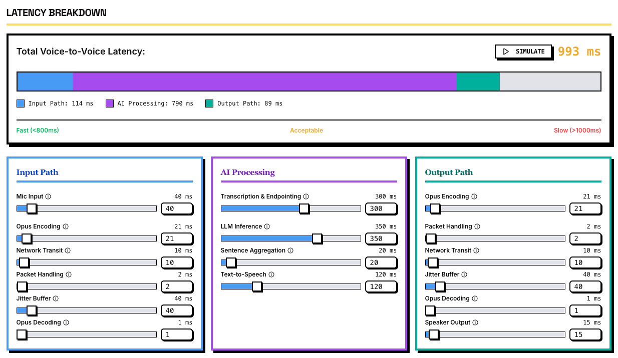
Choose a voice-to-voice latency objective from the task, language, channel, interruption behavior, and user testing; 800 ms is not a universal boundary. Use comparevoiceai.com to explore a timing budget, then replace every stage with measured percentiles from your system.
Speech-to-Text (STT) Optimization
Model Selection for Low Latency
The following table preserves a May 2025 external benchmark snapshot. The links now point to official product information because the old benchmark detail URLs no longer resolve. Re-test current models with one definition of partial and final latency.
| Provider & Model | Latency | Speed Factor |
|---|---|---|
| Whisper Large v3 (Fireworks; historical) | ~300ms | 260 |
| Whisper Large v3 Turbo (Groq) | ~300ms | 252 |
| Universal-2 (AssemblyAI) | ~300ms | 84 |
| GPT-4o Transcribe (OpenAI) | ~320ms | 41 |
Streaming STT can expose interim text before finalization. Provider latency varies by mode, endpointing, region, audio, and load, so treat the table as historical context rather than a target or guarantee.
Streaming Transcription
Rather than buffering the entire user utterance, streaming speech-to-text transcribes audio on the fly. As the user speaks, partial text hypotheses are produced every few hundred milliseconds. This allows the system to get a head start on understanding the query.
Implementation example using the current Deepgram JavaScript SDK pattern:
import { DeepgramClient } from "@deepgram/sdk";

const deepgram = new DeepgramClient({
  apiKey: process.env.DEEPGRAM_API_KEY
});

const connection = await deepgram.listen.v1.connect({
  model: "nova-3",
  language: "en-US",
  smart_format: "true",
  interim_results: "true",
  endpointing: "300"
});

connection.on("message", (event) => {
  if (event.type !== "Results") return;

  const text = event.channel.alternatives[0]?.transcript;
  if (!text) return;

  if (event.is_final) {
    processWithLLM(text);
  } else {
    prepareForLLM(text); // Do not trigger irreversible work from interim text.
  }
});

connection.connect();
await connection.waitForOpen();

// In your capture loop, send each supported audio chunk:
connection.sendMedia(audioChunk);
By the time the user finishes speaking, the agent may already have a useful interim hypothesis. Measure interim and stable-final timing separately, and restrict speculative work to operations that are safe to discard.
Edge Deployment for STT
Edge or on-device STT can remove a cloud round trip, but it still incurs capture, buffering, inference, and device scheduling latency. When using a managed cloud service, place your media ingress or orchestration layer near a supported provider region and measure the complete path.
Scenario: A call center using managed Deepgram Nova-3 cannot deploy that service inside its own data center. It can colocate its application and telephony ingress near an available Deepgram region, compare regional routes, and measure the change. A self-hosted STT model is a separate operational choice.
LLM Optimization Strategies
Model Selection for Real-Time Voice
For real-time dialogue, not all LLMs are created equal. Time-to-First-Token (TTFT) is crucial:
| LLM Model | TTFT | Throughput | Notes |
|---|---|---|---|
| GPT-4o (OpenAI) | ~0.4-0.55s | 117+ tokens/s | Multimodal, excellent for voice |
| Gemini 2.5 Flash (Google) | 0.39s | 268 tokens/s | Ultra-fast, cost-efficient |
| Claude 3.5 Sonnet (Anthropic) | ~0.6s | ~85 tokens/s | Huge context window |
| Mistral 7B (self-hosted; historical) | ~0.13s | ~170 tokens/s | May 2025 benchmark context |
The table is a May 2025 snapshot and mixes model and serving conditions. Establish a TTFT budget from end-to-end user testing, then measure current endpoints at p50, p90, and p99. Sub-500 ms is an illustrative target, not a general requirement or expected result.
Semantic Caching
Semantic caching stores previous queries and LLM answers so that semantically similar prompts can reuse results without a full model call. Unlike traditional key-value caching (which hits only on exact string matches), semantic caching uses embeddings to match queries by intent, not exact wording.
How it works:
- Convert incoming prompt into a vector embedding
- Perform a similarity search in a vector database
- If a similar query is found above threshold, return cached answer
- Otherwise, generate new response and add to cache
A cache hit can avoid a full LLM run, but lookup time and hit rate depend on the embedding, index, network, threshold, and validation policy. Instrument cache lookup and false-hit quality rather than assuming a fixed 50-200 ms result.
Implementation example using LangChain's current MongoDB Atlas semantic-cache integration:
import os

from langchain_core.globals import set_llm_cache
from langchain_mongodb.cache import MongoDBAtlasSemanticCache
from langchain_openai import ChatOpenAI, OpenAIEmbeddings

# Create the Atlas Vector Search index before enabling this cache.
set_llm_cache(MongoDBAtlasSemanticCache(
    connection_string=os.environ["MONGODB_ATLAS_URI"],
    database_name="voice_agent",
    collection_name="llm_cache_v1",
    index_name="vector_index",
    embedding=OpenAIEmbeddings(model="text-embedding-3-small"),
    score_threshold=0.85,
))

llm = ChatOpenAI(
    model=os.environ["OPENAI_CHAT_MODEL"],
    temperature=0,
)

response = llm.invoke("What are your support hours?")
Tune the threshold on evaluated queries, version or isolate the cache when prompts and policies change, and do not reuse personalized or side-effecting answers across users.
Context Management
Feeding long conversation histories or verbose prompts into an LLM is a major source of latency. The more tokens the model must process, the longer it takes to produce a response.
Strategies for prompt optimization:
- Rolling Context Windows:
A simple heuristic is to include only the last N turns of dialogue verbatim, and omit or summarize older turns. This creates a sliding window that "forgets" distant history except for a synopsis.
- Prompt Summarization:
Rather than resending the entire chat history each turn, distill older turns into a concise summary. For example, after a few exchanges, a voice agent can replace the detailed transcript of earlier dialogue with a one-sentence summary or extracted facts.
Code Example for context management:
function preparePrompt(conversation, currentQuery) {
  const recentTurns = conversation.slice(-4); // Keep last 4 turns verbatim

  // If we have older history, summarize it
  let contextPrompt = "";
  if (conversation.length > 4) {
    // Either keep a pre-generated summary, or generate one on demand
    contextPrompt = `Previous conversation summary: ${conversation.summary}`;
  }

  return {
    system: "You are a helpful voice assistant...",
    context: contextPrompt,
    messages: recentTurns,
    currentQuery: currentQuery
  };
}
Developers often keep the most recent user question and agent answer in full (since they're directly relevant), and progressively trim earlier content. This dynamic prompt trimming ensures the prompt doesn't grow past the model's context length.
Connection and Startup Optimization
Reuse supported HTTP, WebSocket, or realtime connections so DNS, TLS, authentication, and session setup do not sit on the critical turn path. Load local configuration, tools, and deterministic greeting audio before the first user request where practical.
Do not send dummy "ping" prompts to try to warm a managed LLM: they add cost and do not establish prompt-cache eligibility for the real request. If a provider documents prompt caching, structure repeated qualifying prefixes according to that model's current rules and measure the actual cache status and latency.
Text-to-Speech (TTS) Optimization
Model Selection for Low Latency
For a voice agent, key metrics are: naturalness, low latency (fast TTFT), fast generation (so speech keeps up with real-time), and customization.
| TTS Engine | TTFT | Characters/s | Notes |
|---|---|---|---|
| Polly Long-form (AWS) | ~100ms | 382 | Historical benchmark |
| Flash v2.5 (ElevenLabs) | ~75ms | 366 | Historical benchmark |
| GPT-4o Mini TTS (OpenAI; now deprecated) | ~200ms | ~20+ | Historical benchmark only |
| Azure Neural (Microsoft) | ~300ms | 252 | Historical benchmark |
| Sonic English (Cartesia; discontinued, replaced by Sonic 3.5) | ~100ms | 41 | Historical benchmark only |
These are May 2025 benchmark values, not current provider guarantees. Measure first audible audio, not only server TTFB, for the active model, region, format, and text length.
Streaming TTS
Streaming text-to-speech is the counterpart to streaming STT. Instead of waiting for the full generated sentence, advanced TTS systems can start synthesizing audio from the first chunk of text and continue as more text comes in. This means as soon as the LLM produces a few words, the agent's voice can start speaking them.
Streaming playback pattern:
// Pseudocode: use the provider's current streaming endpoint and request a
// documented streamable format, such as framed PCM.
const response = await requestTTSStream({ text, format: 'pcm_24000' });
const reader = response.body.getReader();
const decoder = createStreamingDecoder({ format: 'pcm_24000' });

while (true) {
  const { done, value } = await reader.read();
  if (done) break;

  // The decoder must retain incomplete frames between network chunks.
  const audioFrames = decoder.push(value);
  playbackQueue.enqueue(audioFrames);
}

playbackQueue.enqueue(decoder.flush());
Do not call decodeAudioData() independently on arbitrary network chunks: chunk boundaries need not contain complete audio files or codec frames. Use the provider SDK, a streaming decoder, Media Source Extensions where supported, or an AudioWorklet/PCM queue appropriate to the returned format.
The overlap of LLM and TTS is crucial: if the model streams at (say) 20 tokens/sec and the TTS can synthesize just as fast, the spoken output will closely trail the model's generation.
Word-Level Timestamps and Interruption Handling
For conversational voice use cases, being able to track what text the user heard is important for maintaining accurate conversation context. This requires that a model generate word-level timestamp metadata in addition to the audio, and that the timestamp data be reconstructible backwards to the original input text.
This capability is crucial for handling user interruptions:
The instant the user starts speaking while the agent is talking, the agent should stop its speech. This is table stakes for natural dialogue – we've all experienced voice systems that annoyingly keep talking even when we're trying to interject; that's what to avoid.
Example implementation for interruption handling:
// Detect user speech with VAD (Voice Activity Detection)
async function setupVAD() {
  const sileroVAD = await SileroVAD.create();

  // Process audio chunks in real-time
  audioStream.on('data', async (audioChunk) => {
    const isSpeech = await sileroVAD.process(audioChunk);

    // If we detect speech while TTS is playing, interrupt
    if (isSpeech && ttsIsPlaying) {
      stopTTS();  // Immediately stop audio output

      // Use word timestamps to know exactly what was heard
      const lastSpokenWord = getLastSpokenWordFromTimestamps();
      updateConversationContext(lastSpokenWord);

      // Start processing the new user input
      startSTT();
    }
  });
}
Pipeline Optimization for End-to-End Latency
Parallel Processing and Streaming
Modern real-time architectures use streaming at each stage, overlapping tasks to eliminate idle gaps. The goal is to make the conversation feel fluid, as if the agent is listening and formulating a response almost simultaneously.
The key is to process everything in parallel streams:
- Stream audio to STT in real-time
- Stream partial transcripts to LLM as they become available
- Stream LLM tokens to TTS as they're generated
- Stream TTS audio to the user
Overlapping stages can reduce idle time, but only speculate on work that is safe to discard. Unstable partial transcripts should not trigger tool calls, purchases, messages, or other irreversible actions. Measure the complete path at production concurrency rather than inferring an end-to-end result from component benchmarks.
Edge Deployment and Regional Routing
Even the best-optimized model will suffer if every request has to travel long distances across the internet or contend with network variability. For voice AI, which often interfaces with telephony or edge devices, minimizing network latency is crucial.
Key strategies include:
- Measure the complete service path:
Reducing unnecessary network hops can help, but putting every service in one named region is not always possible or optimal. Telephony ingress, provider routing, data residency, failover, and regional model availability determine the actual path.
- Regional routing:
For a geographically distributed workload, compare centralized and regional deployments using actual user, carrier, and provider routes. The geographically nearest application region need not produce the shortest or most reliable end-to-end path.
Evaluation pattern: Compare a centralized deployment with candidate regional deployments using users' actual network paths. Include provider-region availability, data residency, failover, and cross-region dependencies; the improvement must be measured rather than assumed to exceed 100 ms or meet an 800 ms total.
Network Protocol Optimization
Choose transport from the client, network, media, security, and infrastructure requirements. WebRTC is often a strong fit for interactive browser or mobile media because its stack includes congestion control, jitter handling, NAT traversal, and media-oriented audio features. That does not make it universally faster or simpler.
Transport trade-offs:
- WebRTC: media-oriented behavior and browser support, with additional signaling, NAT traversal, and operational complexity
- WebSockets or streaming RPC: often suitable for server-controlled or server-to-server streams, but behavior under packet loss and buffering must be tested
- HTTP streaming: can be appropriate when supported by the provider and intermediaries; avoid repeated polling on the critical path
Benchmark candidate transports under representative loss, jitter, proxies, mobile handoffs, and concurrency. Keep authentication, cancellation, backpressure, and observability in the comparison.
Advanced Techniques for Ultra-Low Latency
Speculative Decoding
A cutting-edge technique to accelerate LLM output is speculative decoding. This involves using a small, fast "draft" model to predict tokens ahead of time, and then having the large model verify or correct them.
Essentially, the draft model generates a chunk of text quickly, and the main model jumps straight to processing that chunk in one go instead of generating token by token. If the draft was correct, the large model just accepts it, achieving a speedup; if not, it falls back to normal generation for that part.
Research suggests speculative decoding can yield 2–3× faster generation on average, and some real-world tests have seen up to 6× improvements in throughput.
Continuous Batching with vLLM
For self-hosted LLMs, continuous batching significantly improves inference performance:
Projects like vLLM, FasterTransformer, and DeepSpeed-Inference are designed to serve LLMs efficiently. They support features like continuous batching, optimized memory management, and multi-threaded decoding.
For example, vLLM introduces a "continuous batching" scheduler that can merge incoming requests on the fly to keep GPUs busy, and uses a unified memory pool for model KV cache to avoid duplication. In their recent update, the vLLM team achieved up to 2.7× higher throughput and 5× lower latency per token on Llama models by such optimizations.
Quantization for Edge Deployment
As mentioned, quantizing a model from 16-bit to 4-bit can drastically reduce memory and computation, allowing it to run faster on the same hardware. This can be done with minimal impact on model quality if done carefully.
For edge scenarios where GPU memory is limited, quantization might be the difference between running a model at all versus not. Additionally, optimizations like compiling the model (via TensorRT, ONNX Runtime, or TVM) can speed up inference by 2× or more.
Scenario: A smart home device manufacturer wants to add voice AI capabilities that work offline. By quantizing a 7B parameter model to 4-bit precision and optimizing with ONNX Runtime, they can run it on an embedded GPU with under 4GB of memory, achieving 20 tokens/second throughput - fast enough for responsive voice interaction without cloud dependency.
Measuring and Monitoring Latency
It's worth learning how to accurately measure latency — from the end user's perspective — if you are building voice AI agents.
You will often see AI platforms quote latencies that are not true "voice-to-voice" measurements. This is generally not malicious. From the provider side of things, the easy way to measure latency is to measure inference time. So that's how providers get used to thinking about latency. However, this server-side view does not account for audio processing, phrase endpointing delay, network transport, and operating system overhead.
How to measure voice-to-voice latency:
Measuring voice-to-voice latency is easy to do manually. Simply record the conversation, load the recording into an audio editor, look at the audio waveform, and measure from the end of the user's speech to the beginning of the LLM's speech.
For automated monitoring:
- Instrument each component with timing logs
- Track p50, p90, and p99 latencies to catch outliers
- Set up alerts when latency exceeds thresholds
- Test with real network conditions and various user scenarios
Conclusion
Achieving human-like latency in voice AI requires optimization at every level - from audio capture to speech synthesis, with careful attention to model selection, streaming processing, context management, and infrastructure.
The most effective strategies include:
- Using streaming APIs for STT, LLM, and TTS
- Selecting models optimized for low TTFT and high throughput
- Implementing semantic caching for common queries
- Managing context effectively to minimize token processing
- Optimizing the measured user-to-provider network path
- Choosing and testing a transport appropriate to the channel
- Implementing efficient interrupt handling
By applying and measuring these optimizations, voice AI developers can work toward the latency target appropriate for their application without treating any threshold as a guarantee.